Un-Expected Threat
July 22, 2021
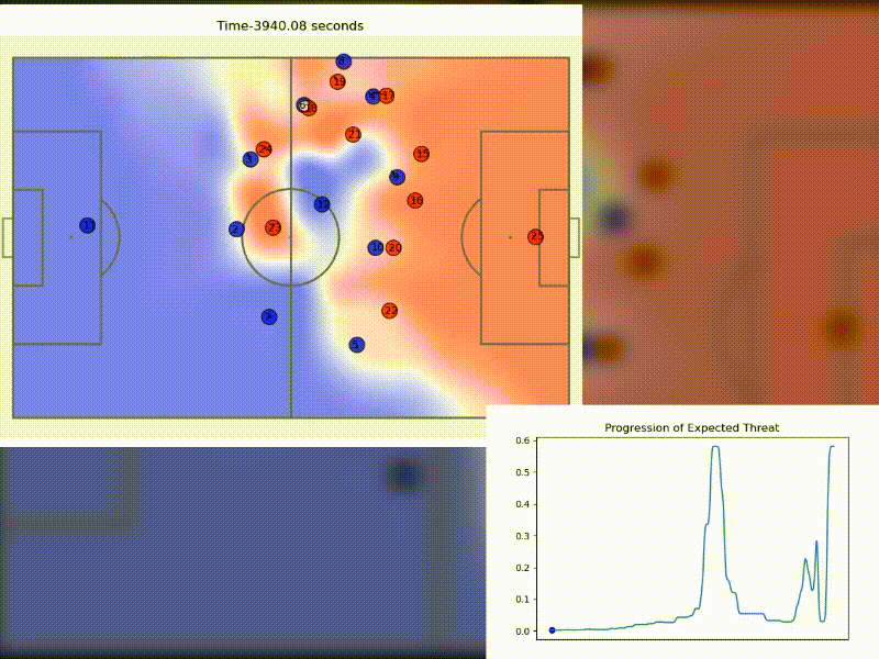
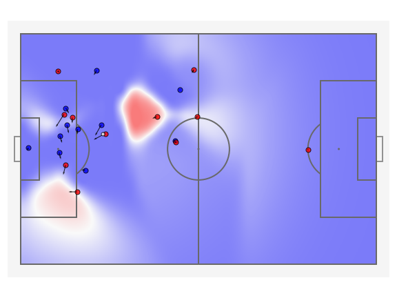
This article aims to bring together the concepts shown above. On left we can see the potential pitch control field (PPCF) (Spearman 2018) for an attack which resulted in a goal, the blue regions represent the portion of the field controlled by the team in blue and the regions marked in red are controlled by the team in red. We can see how the runs of different players influence this region of control, a player running away from a region does not have control over it despite its proximity.
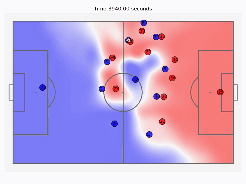
The graph shows the progression of Expected Threat according to the location of the ball on the pitch. The regions closer to the goal have higher values of ‘threat’. More on this later. Expected threat was introduced by Karun Singh in his blog post and is derived with the help of events data. With the help of tracking data we can do better.
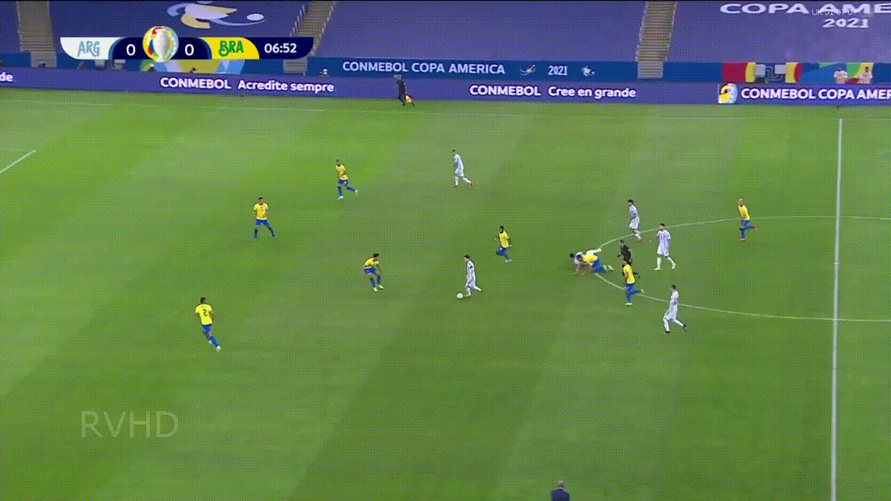
The situation above occurred in the recently concluded Copa America Final. Messi receives the ball in a seemingly decent position but has no passing options and is crowded out soon enough. This further highlights the importance of providing passing lanes to the player who currently has possession. All the passing options are also not equally valuable, a player providing a through ball which might result in a clear goal scoring opportunity should be weighed and rewarded accordingly. The rest of this post will focus on merging the existing models to create a framework which can help us quantify the value of different passing options.
DATA
Tracking data for football matches is not easily available in the public domain. I used the tracking data provided by Metrica Sports which contains a dataset of all events and the positions of all players and the ball recorded at 25Hz for three matches. The event and tracking datasets are synchronised, the information about the players involved in an event is also provided. The data has been anonymized by the provider. I smoothed the tracking data by performing least-squares smoothing to reduce noise as well as calculate the instantaneous higher order derivatives, velocity and acceleration. I also used the openly available wyscout events dataset for the 2017-2018 La-Liga season.
METHOD
I’ll try to explain the methods used in the model by Spearman while pointing out implementation differences that I adopted.
To quantify the danger of a player not in possession of the ball, we need to calculate the probability of that player receiving a pass and the threat he can cause once in possession of it. A successful pass entails two things:
Transition = The probability \((T_{r})\) of the ball moving to an arbitrary point \(\overrightarrow{r}\), within the domains of the legally allowed field.
Control = The probability \((C_{r})\) of the team in possession retaining the ball if it is moved to point \(\overrightarrow{r}\).
Hence the probability of a successful pass (P) at any given game state (D) is:
\(P(P\mid D)\) = \(\sum_{r \in \mathcal{R}}P(C_{r}\cap T_{r}\mid D)\)
This is equivalent to:
\(P(P\mid D)\) = \(\sum_{r \in \mathcal{R}}P(C_{r}\mid T_{r},D)P(T_{r}\mid D)\)
CONTROL MODEL
The original model by Spearman calculates the probability that a team will be able to control possession given the ball is transitioned there \(P(C_{r}\mid T_{r},D)\). Intuitively the longer a player is in proximity to the ball the higher is his probability of controlling the ball. Differing from the original model I chose to ignore the aerodynamic drag faced by the ball. Thus the time taken by the ball to reach an arbitrary point \(\overrightarrow{r}\) is calculated as the distance the ball has to travel divided by the average ball velocity \((15 m/s)\). The time of intercept is defined as the time taken by a player to reach the location of the ball. The maximum velocity of \(5 m/s\) and a constant acceleration of \(7 m/s^{2}\) is assumed for each player. The differential equation as defined in the original model to calculate the control probability of each player at a specified time is given by:
\[\frac{dPPCF_{j}}{\mathbf{dT}} = (1 - \sum_{k }PPCF_{k}(t, \overrightarrow{r}, T \mid s,\lambda_{j}))f_{j}(t,\overrightarrow{r},T \mid s)\lambda_{j}\]The parameter \(\lambda_{j}\) is the rate of control, i.e. inverse of the mean time that a player takes to make a controlled touch. I used the values \(1\) for attackers and \(1.72\) for defenders as in the original model. This takes into account the fact that a defender can easily boot the ball out of play whereas the attacker need to take a controlled touch to further the attack. The \(\lambda_{j}\) value for players who are in an offside position is set to zero.
\(f_{j}(t,\overrightarrow{r},T \mid s)\lambda_{j}\) represents the probability that player \(j\) at time \(t\) can reach the location \(\overrightarrow{r}\) within some given time \(T\). This is calculated as: \(f_{j}(t,\overrightarrow{r},T \mid s)\lambda_{j} = [1+e^{-\pi\frac{T-t_{exp}(t-\overrightarrow{r})}{\sqrt3\ s}}]^{-1}\), the CDF of logistic distribution. The parameter \(s\) is equal to 0.45.
TRANSITION
The probability of passing a ball accurately should decrease as the distance increases. On an average the distribution of displacements between subsequent on ball events is normally distributed. In addition to this it is expected that a player will pass to a region where the probability of losing possession is low, this has already been calculated in the Control Model. By superimposing these models we create a probability decision field.
\[P(T_{r}\mid D) = N(\overrightarrow{r},\overrightarrow{r_{b}}(t),\sigma)[\sum_{k \in \mathcal{A}}PPCF_{k}(t,\overrightarrow{r})]^{\alpha}\]This equation is further normalized to unity (this makes sure that the ball is passed to some place).
I used the same parameters as done in the original work. The original model also assumes that this probability remains the same irrespective of the time the player has in possession.
By combining both the transition and control models we can find the probability of the player in possession passing the ball to any location \(\overrightarrow{r}\).
\(P(P\mid D)\) = \(\sum_{r \in \mathcal{R}}P(C_{r}\mid T_{r},D)P(T_{r}\mid D)\)
EXPECTED THREAT
Simply put it is the probability of scoring a goal within the next \(m\) events from any point on the field. Here \(m\) is a variable and can be changed. Details about the derivation can be found in the original blog post. We essentially divide the field into \(k\) zones, and then iteratively calculate the expected threat value until convergence.
\[xT_{x,y} = (s_{x,y}\times g_{x,y}) + (m_{x,y}\times \sum_{z=1}^{M} \sum_{w=1}^{N} T_{(x,y)\rightarrow (z,w)}xT_{(z,w)})\]Here \(M\) and \(N\) are the number of zones along the \(x\) and the \(y\) axes respectively.
I computed \(xT\) matrix using all the events data for the 2017-2018 La-Liga season in the wyscout dataset for \(5\) iterations.
BETTER DATA BETTER MODELS
By combining both these models we can find the Probability of scoring within the next \(5\) actions at any position on the field. This is obviously a simplifying assumption as the threat of a position should also be dependent on the game state. Like Spearman I believe that has been factored in the model to some extent by using the PPCF values. Hence I have replaced \(P(S_{5}\mid C_{r},T_{r},D)\) with \(P(S_{5}\mid C_{r},T_{r})\) thus ignoring the game state D.
\(P(S_{5}\mid D)\) = \(\sum_{r \in \mathcal{R}}P(S_{5}\mid C_{r},T_{r})P(C_{r}\mid T_{r},D)P(T_{r}\mid D)\)
We get a probability density field which can be integrated over the football field to find the probability of scoring within the next six events at any particular point of time.
If looked at closely, this is similar to the Expected Threat model. Instead of assuming a constant Transition matrix we have calculated it based on the current state of the game. The only option provided to the player is to ‘pass’ the ball, hence this is a good quantification of the quality of passes available at any point of time but does not reflect the overall threat posed. To achieve that we will need to calculate the probability of taking a shot at any position \(r\). This should be a function of the distance from the goal. A player is also more probable to take a shot if he gets more time on the ball and the passing options are not lucrative enough. The probability of scoring can be calculated with the help of an expected goals model trained on events dataset. Sadly to find the parameters involved we would need a larger training dataset and hence I constrain this to only passing options for now.
In this article ‘threat’ corresponds to the threat posed by the passing options available only, In most cases this will be equivalent to the overall threat of the situation as the probability to shoot and score a goal is small unless a player is reasonably close to the goal.
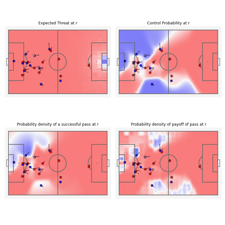
a) The Expected Threat at r (this is constant irrespective of the match situation). b) Control Probability at r. c) Probability density of completing a successful pass at r, high where the region is controlled by the team in possession as well as the distance is less. d) Probability density of the payoff of a pass at r, the model is able to successfully factor in the importance of the through ball to the right wing despite it not being a region where a successful pass is probable.
On integrating over the whole field we can find the probability of the next event being a successful pass is equal to \(80\)%. Whereas the probability of scoring within the next \(6\) events is \(0.04\)%.
Note - The xT values were calculated for a total of 300 zones and hence underestimates the threat in most cases. This can easily be rectified with the help of dividing the field into more zones.
CONTINUOUS DECISIONS
With the method explained above we can calculate the ‘threat’ of a position at any point of time. Spearman considers only the game state at the timestamp of the event. But this fails to reward players who might have been in a ‘good’ position some time before the player actually played the pass. That player might now be in an offside position and hence the threat he poses is nil. To counter this we can sum the threat values for the whole duration in which a team was in possession of the ball during an attack. This is also particularly useful for comparing the quality of two different attacks. The value of this sum no longer represents a ‘probability’ value. For individual players a larger value of sum represents higher ability of providing a dangerous passing option over a longer period of time.
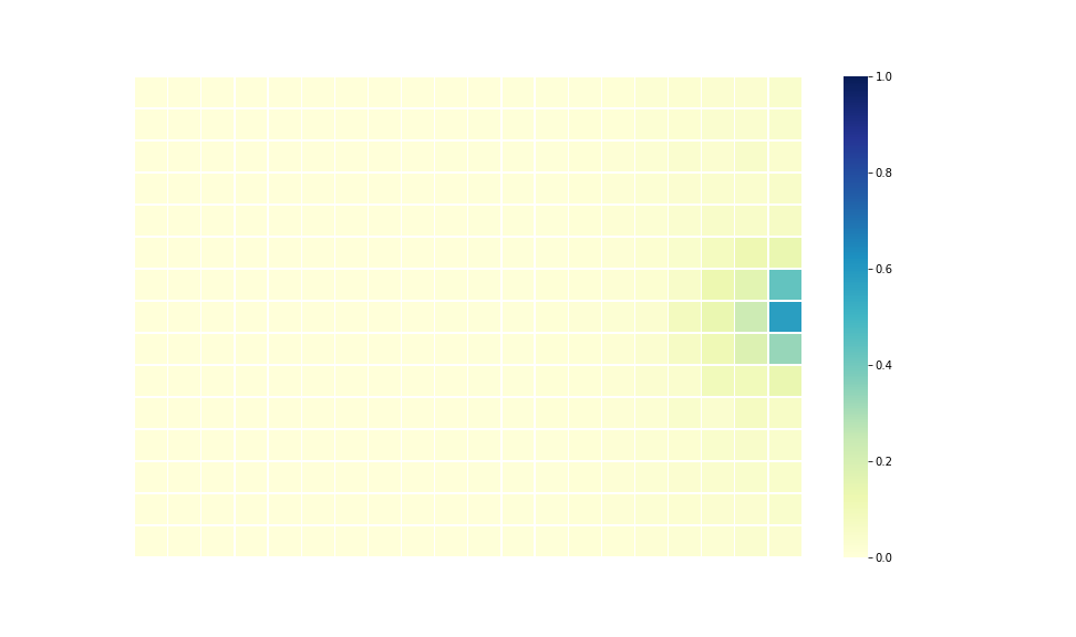
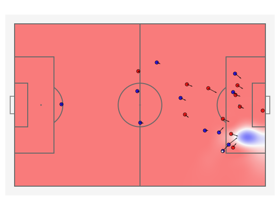
This is the probability density field of a successful pass, we can see that the contribution of the player on the right wing has been ignored because he is in an offside position, any analysis done taking into consideration only this timestamp will not reward the player appropriately even though he might have been in an onside position earlier.
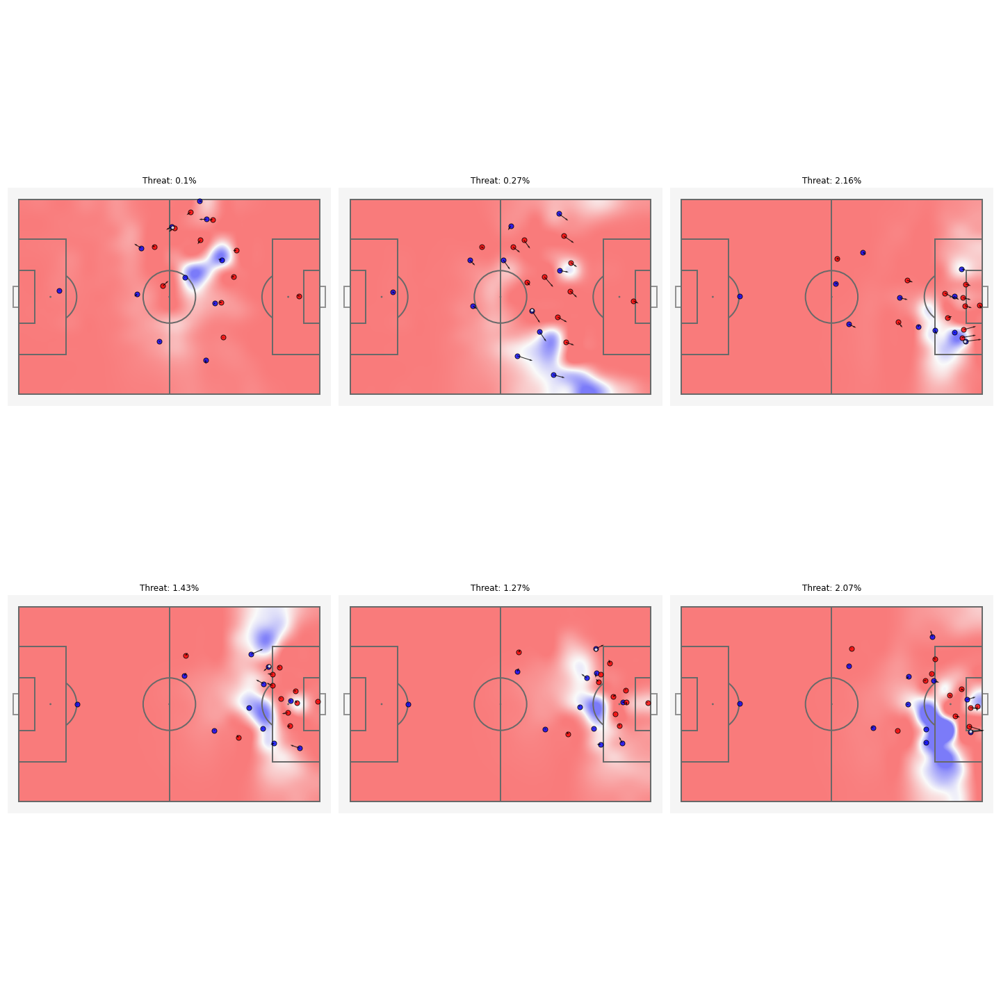
The attack leading up to the goal along with the control field values at all times.
Below are the timestamps for all the passes played in the attack shown above along with the threat probability density field. We can judge the decision making of different players by seeing if the overall threat increased or decreased after each successive event, we can also visualise the pass with the highest payoff for each timestamp. This shows us that the attempted cross by number \(5\) was a wrong decision as a cutback would have been more rewarding.
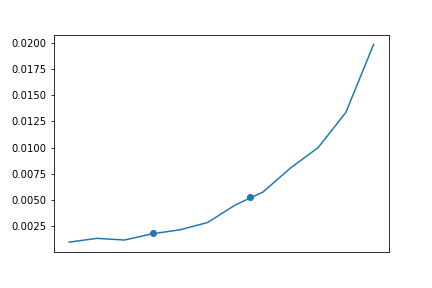
I calculated the threat for the attack leading up to the attempted cross in order to further quantify its quality. I used a rather large time step of one second, shorter time-steps should be used for improved accuracy. A plot showing the threat progression can be seen below. The points represent the change of possession of a player. This also puts into perspective the quality of dribble which helped hold and further advance the ball while giving time to players to get into a better position. Calculating the threat for some time period leading up to the attack can help make better opinions about the players and is a better estimate of the quality of the whole attack.
INDIVIDUAL CONTRIBUTIONS
This is the threat probability density field for player \(7\), the value of threat posed by the player is \(0.05\). Even though he never receives the ball, his run opens up the space for number \(5\) to dribble and hence is instrumental in the attack. By summing the threat value for an individual player for a duration \(N\) of the attack we can find his overall contribution as well.
CONCLUSION
With the help of the existing models we can create a framework which is able to quantify the quality of each passing option available. We can further weigh the importance of the off ball runs of different players involved in the attack by calculating the percentage of threat posed by them. This can also be used to reward the on the ball actions by the threat created by a pass. Comparing all the 11 players involved in an attack irrespective of whether they were ever in possession of the ball is also possible.
The code for everything discussed in this post can be found here, my derivation of Expected Threat. Structured and probably more efficient code for calculating PPCF and more can be found on the Friends of Tracking github.
REFERENCES
2) https://www.researchgate.net/publication/327139841_Beyond_Expected_Goals